Mastering Linear Regression: From Scratch with Gradient Descent Only.

Introduction

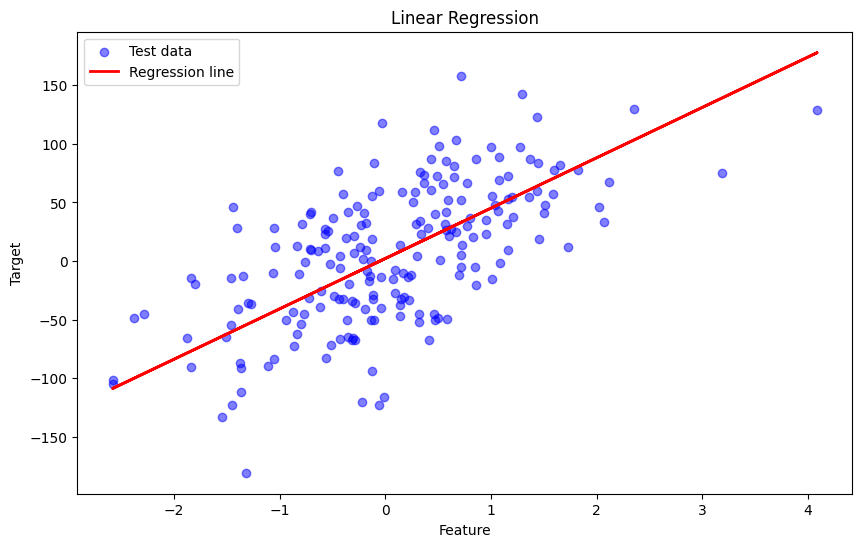
Linear Regression is a method in which we tries to best-fit a line on the dataset in a way that that minimizes the mean square error. In other words Linear Regression is a method used to define a relationship between a dependent variable (Y) and independent variables (x1, x2, ..., xk). Which is simply written as :

\[ \hat{y} = {m_1}\times{x_1} + {m_2}\times{x_2} + \ldots + {m_k}\times{x_k} + b \] or simply \[ \hat{y} = {M}{X} + b \]

where:

• ŷ is the predicted value (dependent variable).
• X is the independent variables.
• M is the slope of the line (weights).
• b is the y-intercept (bias).

Example Scenario

Imagine we wants to predict the house price based on some parameters like rooms and area etc. Then we could establish a relationship between its price and the input parameters using linear regression algorithm.

Section 2: Mathematical Foundations

Mean Squared Error (MSE)

To measure the error of our linear regression model, we use the Mean Squared Error (MSE), which calculates the mean of the squared difference between the actual and predicted values:

\[ \text{MSE} = \frac{1}{n} \sum_{i=1}^{n} (y_i - \hat{y_i})^2 \]

where:

• n is the number of data points.
• y𝒊 is the actual value.
• ŷ𝒊 is the predicted value.

On Now you know what mean squared error is but we want to minimize this error to accurately fit the line on the data points. but how to minimize this error?

Gradient Descent

Gradient descent is an algorithm used to minimize the cost function (here MSE) by iteratively updating the model's parameters (slope m and intercept b). Gradient descent uses the following rules to calculate the new parameters:

\[ m' = m - \alpha \frac{\partial \text{E}}{\partial m} \] \[ b' = b - \alpha \frac{\partial \text{E}}{\partial b} \]

where:

• α is the learning rate.
• E is the cost function (here MSE).
• dE/dm and dE/db are the partial derivatives of the cost function with respect to m and b.

Partial Derivatives

The partial derivatives of the MSE with respect to m:

\[ \frac{\partial \text{MSE}}{\partial m} = \frac{1}{n} \sum_{i=1}^{n} (y_i - \hat{y_i})^2 \] \[ \frac{\partial \text{MSE}}{\partial m} = \frac{1}{n} \sum_{i=1}^{n} (y_i - (m {x_i} + b))^2 \] \[ \frac{\partial \text{MSE}}{\partial m} = \frac{1}{n} \sum_{i=1}^{n} (y_i - (m {x_i} + b))(-2{x_i}) \] \[ \frac{\partial \text{MSE}}{\partial m} = -\frac{2}{n} \sum_{i=1}^{n} x_i (y_i - (m {x_i} + b)) \] \[ \frac{\partial \text{MSE}}{\partial m} = -\frac{2}{n} \sum_{i=1}^{n} x_i (y_i - \hat{y_i}) \]

The partial derivatives of the MSE with respect to b:

\[ \frac{\partial \text{MSE}}{\partial b} = \frac{1}{n} \sum_{i=1}^{n} (y_i - \hat{y_i})^2 \] \[ \frac{\partial \text{MSE}}{\partial b} = \frac{1}{n} \sum_{i=1}^{n} (y_i - (m {x_i} + b))^2 \] \[ \frac{\partial \text{MSE}}{\partial b} = \frac{1}{n} \sum_{i=1}^{n} (y_i - (m {x_i} + b))(-2) \] \[ \frac{\partial \text{MSE}}{\partial b} = -\frac{2}{n} \sum_{i=1}^{n} (y_i - (m {x_i} + b)) \] \[ \frac{\partial \text{MSE}}{\partial b} = -\frac{2}{n} \sum_{i=1}^{n} (y_i - \hat{y_i}) \]

Section 3: Implementing Linear Regression from Scratch in Python

Here's how you can implement linear regression from scratch using Python:

import numpy as np
from sklearn.datasets import make_regression
from sklearn.model_selection import train_test_split
from sklearn.metrics import mean_squared_error, r2_score

X, Y = make_regression(n_samples=10000, n_features=5, noise=50)

X_train, X_test, Y_train, Y_test = train_test_split(X, Y, test_size=0.2)

M = np.random.random(X.shape[1])
b = np.random.random(1)
y = lambda x : (M * x).sum(axis=1) + b
initial_predictions = y(X_test)
initial_mse = mean_squared_error(initial_predictions, Y_test)
initial_r2 = r2_score(initial_predictions, Y_test)
print(f"Initial MSE: {initial_mse:.5f}")
print(f"Initial R^2 Score: {initial_r2:.5f}")

lr = 0.0001
epoch = 100
for epoch in range(epoch+1):
    errors = Y_train - y(X_train)
    dEdM = -2 * errors.dot(X_train)
    dEdB = -2 * errors.mean()
    M -= dEdM * lr
    b -= dEdB * lr
    if epoch % 10 == 0:
        print(f"[{epoch}] ERROR: {mean_squared_error(y(X_test), Y_test):.5f}")

final_predictions = y(X_test)
final_mse = mean_squared_error(final_predictions, Y_test)
final_r2 = r2_score(final_predictions, Y_test)
print(f"Final MSE: {final_mse:.5f}")
print(f"Final R^2 Score: {final_r2:.5f}")

from sklearn import linear_model
sklearn_model = linear_model.LinearRegression()
sklearn_model.fit(X_train, Y_train)
sklearn_predictions = sklearn_model.predict(X_test)
print(f"sklearn MSE: {mean_squared_error(sklearn_predictions, Y_test):.5f}")
print(f"sklearn R^2 Score: {r2_score(sklearn_predictions, Y_test):.5f}")

output

Initial MSE: 22167.29314
Initial R^2 Score: -7556.18751
[0] ERROR: 9424.97606
[10] ERROR: 2473.21239
[20] ERROR: 2472.80553
[30] ERROR: 2472.80154
[40] ERROR: 2472.80166
[50] ERROR: 2472.80185
[60] ERROR: 2472.80204
[70] ERROR: 2472.80222
[80] ERROR: 2472.80241
[90] ERROR: 2472.80260
[100] ERROR: 2472.80279
Final MSE: 2472.80279
Final R^2 Score: 0.87769
sklearn MSE: 2472.89865
sklearn R^2 Score: 0.87769

What Next?

do you realize that to find the minima we can equivate the gradients of the cost function to zero as we know that the gradients of the cost function is zero at maxima or minima. So you can write code for this as equating the gradients to zero is much more efficient then using Gradient Descent.

You can find the code for this approach on my github account. Or you can see this post for guidance.